Nash Equilibria on Parallel Networks with Horizontal Queues

Walid Krichene
Jack Reilly
Saurabh Amin
Alexandre Bayen

Motivation and results

Congestion games: equilibrium behavior of selfish agents on networks
Assumptions unsuitable for phenomena on freeway networks
Approach:
- Derive new class of latencies from traffic theory
- Exactly solve for Nash equilibria in context of congestion games
- Provide practical solutions based on results
- Use as basis for study of partial control
Results:
1. Non-uniqueness of equilibria
2. $O\left(N^2\right)$ solution to Best Nash equilibrium
3. Analytical expression for price of stability on two-link network

Outline

Introduction
- Congestion games
- Two-mode latency functions
- Network and assumptions
Enumerating Nash equilibria
- Definition
- Allowable congestion modes
- Bounding number of equilibria
Best Nash equilibrium (BNE)
- Defining single link, free flow equilibria (SLFF)
- Existence of SLFF equilibrium
- Definition of best Nash equilibrium (BNE)
- Algorithm for BNE
Price of stability for two-link network
- Price of anarchy / Definition
- Solution for our network
- Analysis

Congestion games

Parallel network, $N$ edges (links)
Continuum of players, total flow demand $r$
- Players route themselves "selfishly"
Individual latency $\ell_n(x_n)$ on link $n$ depends on total flow $x_n$.
- Latencies are usually assumed non-decreasing and $x\ell\left(x\right)$ convex.
Total cost: $C(x) = \sum_n x_n \ell_n(x_n)$

Non-decreasing latency functions

Congestion games literature usually assumes a non-increasing latency ($\frac{d\ell}{dx} \ge 0$)
- Unique mapping from flow to latency
Latencies are equal for all occupied links
- All unoccupied have greater or equal latencies
Equilibrium is essentially unique given demand $r=\sum_i x_i$.

Network

New class of latencies: from traffic theory

Because vehicles take up physical space (thus, horizontal queues), density of vehicles is important quantity.
Fundamental Diagram
Density $\rho$ $(\frac{cars}{length})$ $\rightarrow$ Vehicle flow $x$ ($\frac{cars}{time}$)
Single flow $x'$ does NOT have unique density
Two distinct modes
- Free flow $\left(\rho^-\right)$: few cars moving quickly
- Congested $\left(\rho^+\right)$: many cars moving slowly
Can express velocity $v$:
$$ v\left(\rho\right)=\frac{x\left(\rho\right)}{\rho} $$

Constant velocity in free flow

New class: density function to flow mapping

We can derive latency from fundamental diagram $f$ as a function of $\rho$:
$$ \ell\left(\rho\right) \propto v\left(\rho\right)^{-1} = \frac{\rho}{x\left(\rho\right)} $$
Can also express latency as non-unique mapping from flux
Introduce binary variable $m$:
$$ m = \begin{cases} 0 & \text{free flow} \\ 1 & \text{congestion} \end{cases} $$
Then latency can be uniquely determined from flow $x$ and mode $m$...

Two-mode congestion function

\begin{eqnarray} \ell_n: [0, x_n^{\max}] \times \{ 0,1 \} & \rightarrow & \mathbb{R}_+ \\ \left(x_n, m_n \right) & \mapsto & \ell_n = \ell_n\left(x,m\right) \end{eqnarray}

Subject to the following conditions:

$\ell_n( \cdot ,0) = a_n$ constant
$\ell_n(\cdot ,1)$ is decreasing from $(0, x_n^{\max})$ onto $(a_n, +\infty)$
$\lim_{x_n \rightarrow x_n^{\max}} \ell_n(x_n ,1) = a_n$

Assume $a_1 < a_2 < \ldots < a_n$.

Outline

Introduction
- Congestion games
- Two-mode latency functions
- Network and assumptions
Enumerating Nash equilibria
- Definition
- Allowable congestion modes
- Bounding number of equilibria
Best Nash equilibrium (BNE)
- Defining single link, free flow equilibria (SLFF)
- Existence of SLFF equilibrium
- Definition of best Nash equilibrium (BNE)
- Algorithm for BNE
Price of stability for two-link network
- Price of anarchy / Definition
- Solution for our network
- Analysis

Nash equilibria: definition

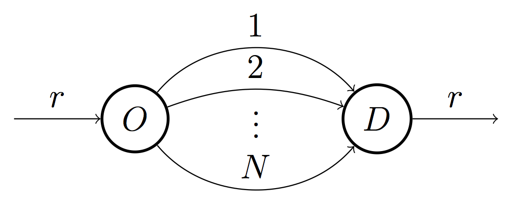
Nash equilibria are any flow assignment such that there is no incentive any flow to switch links.

An assignment $\left(x,m\right)\in\mathbb{R}_+^{N} \times \left\{ 0,1\right\} ^{N}$
for a game instance $\left(N,r\right)$ is a Nash equilibrium, if $$ \forall n: x_n > 0 \Rightarrow \ell_n \left(x_n,m_n\right)\le\ell_k\left(x_k,m_k\right) $$

Nash equilibria: allowable modes

Number of possible modes is combinatoric (exponential in # of links)
For Nash equilibria, can reduce to linear in # of links

If link $k$ is congested, then links $< k$ are also congested

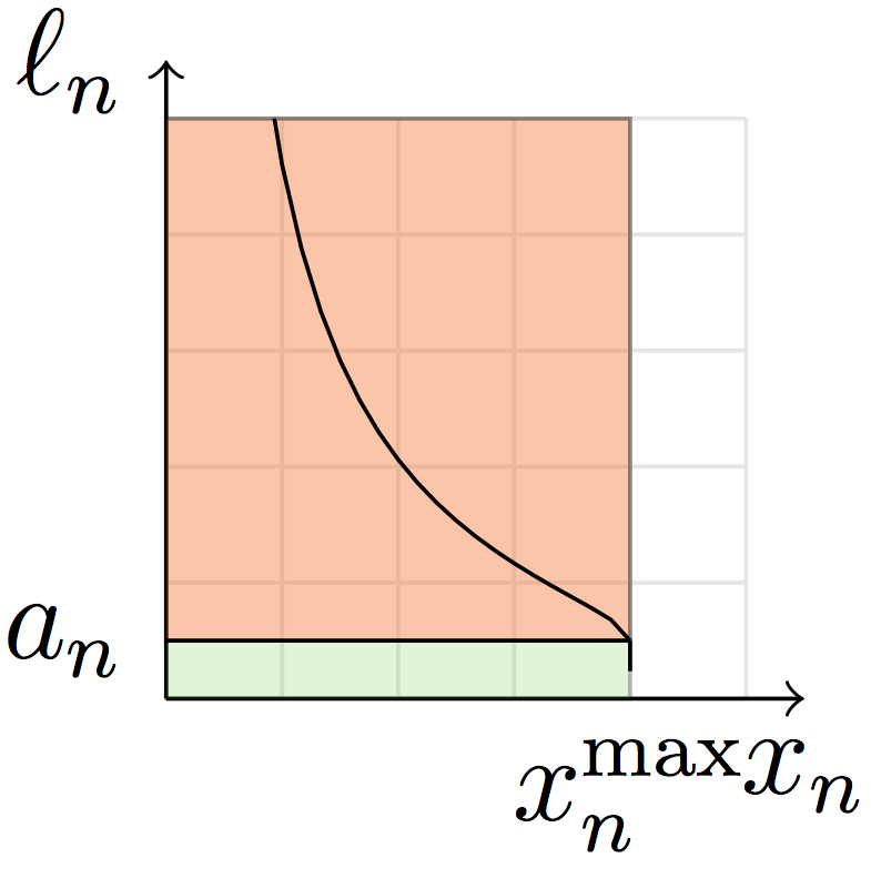
Why?: $\forall j < k, a_j < a_k \le \ell_k \left(x_k, 1\right)$

If link $k$ is in the support and in free flow, then all links $< k$ are congested, and all links $>k$ are not in the support.

Why?: $\forall j > k, a_j > a_k = \ell_k \left(x_k, 0\right)$

For instance $(N, r)$, there are at most $2N$ Nash equilibria.

Outline

Introduction
- Congestion games
- Two-mode latency functions
- Network and assumptions
Enumerating Nash equilibria
- Definition
- Allowable congestion modes
- Bounding number of equilibria
Best Nash equilibrium (BNE)
- Defining single link, free flow equilibria (SLFF)
- Existence of SLFF equilibrium
- Definition of best Nash equilibrium (BNE)
- Algorithm for BNE
Price of stability for two-link network
- Price of anarchy / Definition
- Solution for our network
- Analysis

Single link free flow equilibria (SLFF)

For $1\leq n\leq k\leq N$, congestion flow $\hat{x}_n \left(k \right)$ is the unique flow in $[0,x^{\max}_n]$ that satisfies $$ \ell_{n}(\hat{x}_n \left(k\right),1)=a_{k} $$

$$ \begin{eqnarray} \bar{m}^{k} & := & (1,\dots,1,\overset{k}{0},\dots,0)\\ \bar{x}^{k,r} & := & (\hat{x}_1 \left(k\right), \hat{x}_2 \left(k\right), \ldots, \hat{x}_{k-1}\left(k\right), r-\sum_{n=1}^{k-1}\hat{x}_n\left(k\right), 0, \dots, 0) \end{eqnarray} $$

Existence of SLFF equilibria

If there exists an equilibria, then there exists an SLFF equilibria.

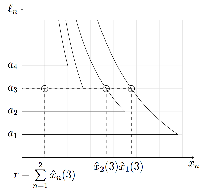
Proof: by induction, iteratively shrink the support

Given any equilibria, there exists an SLFF equilibria with smaller or equal cost.

Network
Latencies

Status:

Best Nash equilibria (BNE)

$$ \text{BNE} \left( N,r \right) = \underset{x,m\in \text{NE}\left(N,r\right)}{\arg \min}C\left(x,m\right) $$

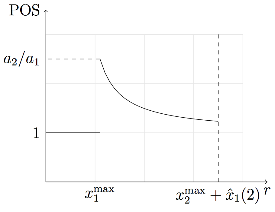
BNE is the equilibrium that minimizes total cost (we can show this to be unique).

The BNE for a network $\left(N,r\right)$ is the SLFF with the smallest support.

Runs in $O\left(N^2\right)$ (NE for non-decreasing latencies requires solution of convex optimization problem)

Procedure $BNE\left(N,r\right)$

$\textbf{Inputs:}$ Size of the network $N$, demand $r$
$\textbf{Outputs:}$ Best Nash equilibrium $(x, m)$
$\quad$for $k \in \{1, \dots, N\}$
$\quad$let $(x, m)$ = freeFlowConfig($k$)
$\quad$if $x_k \in [0, x^{\max}_k]$
$\quad$$\quad$return $(x,m)$
return No-Solution

Procedure $freeFlowConfig\left(k\right)$

$\textbf{Inputs:}$ Free-flow link index $k$
$\textbf{Outputs:}$ Assignment $(x,m)=(\bar{x}_k\left(r\right),\bar{m}_k)$
for $i \in \{ 1, \dots, N \}$
$\quad$if $i < k$
$\quad$$\quad$$x_i = \hat{x}_i\left(k\right)$, $m_i = 1$
$\quad$elseif $i$ == $k$
$\quad$$\quad$$x_i = r - \sum_{n=1}^k x_n$, $m_i = 0$
$\quad$else
$\quad$$\quad$$x_i = 0$, $m_i = 0$
return $(x,m)$

Outline

Introduction
- Congestion games
- Two-mode latency functions
- Network and assumptions
Enumerating Nash equilibria
- Definition
- Allowable congestion modes
- Bounding number of equilibria
Best Nash equilibrium (BNE)
- Defining single link, free flow equilibria (SLFF)
- Existence of SLFF equilibrium
- Definition of best Nash equilibrium (BNE)
- Algorithm for BNE
Price of stability for two-link network
- Price of anarchy / Definition
- Solution for our network
- Analysis

Price of Stability/Anarchy

Price of anarchy (POA) measures inefficiency of NE

For linear, increasing latencies, $POA \le 3/2$ (Roughgarden)

$$ POA\left(N,r\right) = \frac{\underset{x,m\in NE\left(N,r\right)}{\max} C\left(x,m\right)} {\underset{m, \sum x = r}{\min} C\left(x,m\right)} $$

For non-unique NE, price of stability (POS) measure inefficiencies w.r.t. smallest cost NE.

$$ POS\left(N,r\right) = \frac{\underset{x,m\in NE\left(N,r\right)}{\min} C\left(x,m\right)} {\underset{m, \sum x = r}{\min} C\left(x,m\right)} = \frac{BNE\left(N,r\right)}{SO\left(N,r\right)} $$

Social Optimum

$$ SO\left(N,r\right) = \underset{m, \sum x = r}{\min} C\left(x,m\right) $$

Social Optimum is the lowest cost achievable for $\sum x = r$.
For our network, solution is straight-forward:

Start on link with lowest latency
Either:
- Fill until demand is satisfied and Stop
- Fill to maximum capacity of link and move to link with next lowest latency

$m_{SO}=\left(0,0,\ldots\right)$

Social Optimum

BNE

POS for two-link network

For two-link network, closed form solution is easily expressible

$$ \begin{eqnarray} POS\left(2,r\right) & = & \frac{r a_2}{r a_2 - x_1^{\max} (a_2 - a_1)} \\ & = & \frac{1}{1 - x_1^{\max} / r \left( 1-a_1/a_2 \right) } \end{eqnarray} $$

Inefficiencies are very sensitive to changes in demand when links near capacity.
Rerouting a small amount of flow to longer link can have large benefits!

POS: Two Links

Thank you for listening!

Questions?

Nash Equilibria on Parallel Networks with Horizontal Queues

Motivation and results

Outline

Congestion games

Non-decreasing latency functions

Network

New class of latencies: from traffic theory

New class: density function to flow mapping

Two-mode congestion function

Outline

Nash equilibria: definition

Nash equilibria: allowable modes

Outline

Single link free flow equilibria (SLFF)

Existence of SLFF equilibria

Network

Latencies

Status:

Best Nash equilibria (BNE)

Procedure $BNE\left(N,r\right)$

Procedure $freeFlowConfig\left(k\right)$

Outline

Price of Stability/Anarchy

Social Optimum

Social Optimum

BNE

POS for two-link network

POS: Two Links

Thank you for listening!